3D Scenes in the weights of Neural Networks! - Introduction to NeRF and SNeRG
Last Wednesday, I came across an Interesting Paper - “Representing Scenes as Neural Radiance Fields for View Synthesis”. As someone who has dabbled with Blender for a while, I know that 3D scenes would easily take gigabytes in storage, especially if photorealistic. However, the authors found a way to store photorealistic scenes under 5 MB. How did they achieve this?
(Note: This article is pretty long and technical, so I would advise you to have a cup of coffee next to you while reading it. This article explains two interesting papers.)
Neural Radiance Fields (NeRF)
t is a method to synthesize views of a 3D scene, which can be captured through a few photos. We will train one neural network to fit one scene. We will have a 5-dimensional input consisting of (x,y,z) of a particular position in space and a viewing direction (theta,phi), and the network’s output will be (r,g,b) color and the volume density (i.e presence of an object). This function is called the Radiance Field.
To render a Neural Radiance Field from a particular viewpoint and direction
- Send out Camera Rays through the scene to generate a sampled set of 3D Points
- Use these points and viewing direction as input to the neural network, to generate a set of colors and volume densities
- Use Classical Volume Rendering Techniques to accumulate those colors and volume densities into a 2D image.
The process above is differentiable, so we can use our trust-worthy gradient descent.
Scene Representation
The representation is constrained to be multi-view consistent by restricting the network to predict volume density as a function of only the location, while the RGB color is a function of both location and viewing direction.
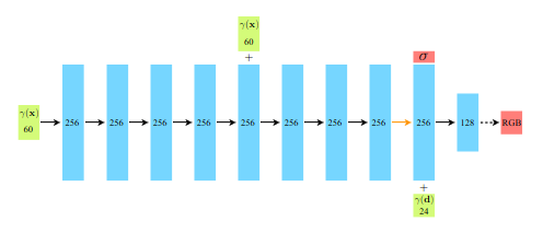
We achieve the above by the following MLP architecture:
- First, only the location is passed as input to the neural network, which is processed by 8 fully connected MLP layers, and each of the 8 layers uses ReLU activation, each with 256 channels.
- The location input is connected to the fifth layer’s activation through a skip connection.
- After the 8 layer an additional layer is present, where we concatenate the viewing direction to the feature vector. This feature vector represents the volume density.
- At the end, we have a sigmoid activation which emits the emitted RGB radiance.
Volume Rendering with Radiance Fields
To render radiance fields, we use techniques from computer graphics. The expected color of a camera ray (r(t) = o + td) can be given by this integral
$$ C(r) = \int_{t_n}^{t_f} T(t)\sigma(r(t))c(r(t),d)dt $$ $$ T(t) = exp(-\int_{t_n}^t\sigma(r(s))ds $$
The function T(t) is the accumulated transmittance along the ray from t_n to t, i.e. the probability that the ray travels from t_n to t without hitting any other particle. Rendering a view requires estimating this integral.
To estimate this, we can use something called the quadrature rule. We need samples to use the quadrature rule. We first partition into evenly spaced regions and then draw a sample uniformly at random from these regions. Using these samples, we can use the quadrature rule resulting in the following equation.
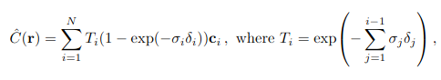
(Source - NeRF: Representing Scenes as Neural Radiance Fields for View Synthesis - https://arxiv.org/pdf/2003.08934)
Here T_i is the alpha value.
To know more about the techniques mentioned in the section. you can have a look at these:
- Ray Tracing Volume Densities - https://dl.acm.org/doi/pdf/10.1145/964965.808594
- Introduction to Numerical Integration - https://math.libretexts.org/Workbench/Numerical_Methods_with_Applications_(Kaw)/7%3A_Integration/7.01%3A_Prerequisites_to_Numerical_Integration
Optimising a Neural Radiance Field
Neural networks rarely achieve the performance desired without extra tweaking. This statement holds true in the case of NeRFs also. The inputs if given as it is, result in the network not converging even after training for a long time. This is because neural networks are biased toward learning lower-frequency functions. They perform poorly at representing high-frequency variation.
We want to map our inputs to a higher dimensional space, therefore we use the following encoding function to map to higher dimensions.
$$\gamma(p) = (sin(2^0\pi p),cos(2^0\pi p),..,sin(2^{L-1}\pi p),cos(2^{L-1}\pi p))$$
L is just a value found through experimentation.
When we render, evaluating our network at N points along each camera ray is inefficient, as we spend time computing stuff in free space and regions blocked by objects. Thus by drawing inspiration from early works of Volume Rendering, a hierarchical approach is used.
Two networks are optimized per scene. One network is “coarse” and another is “fine”. Compute color from the “coarse” network. You could rewrite the color as follows:
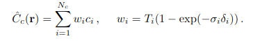
(Source - NeRF: Representing Scenes as Neural Radiance Fields for View Synthesis - https://arxiv.org/pdf/2003.08934)
If we normalize the weights, we will get a Probability Density Function. We can sample a second set of locations from this distribution using inverse transform sampling, and then evaluate our fine network at the union of the first and second sets of samples.
These tweaks allow the MLP network to converge much more easily.
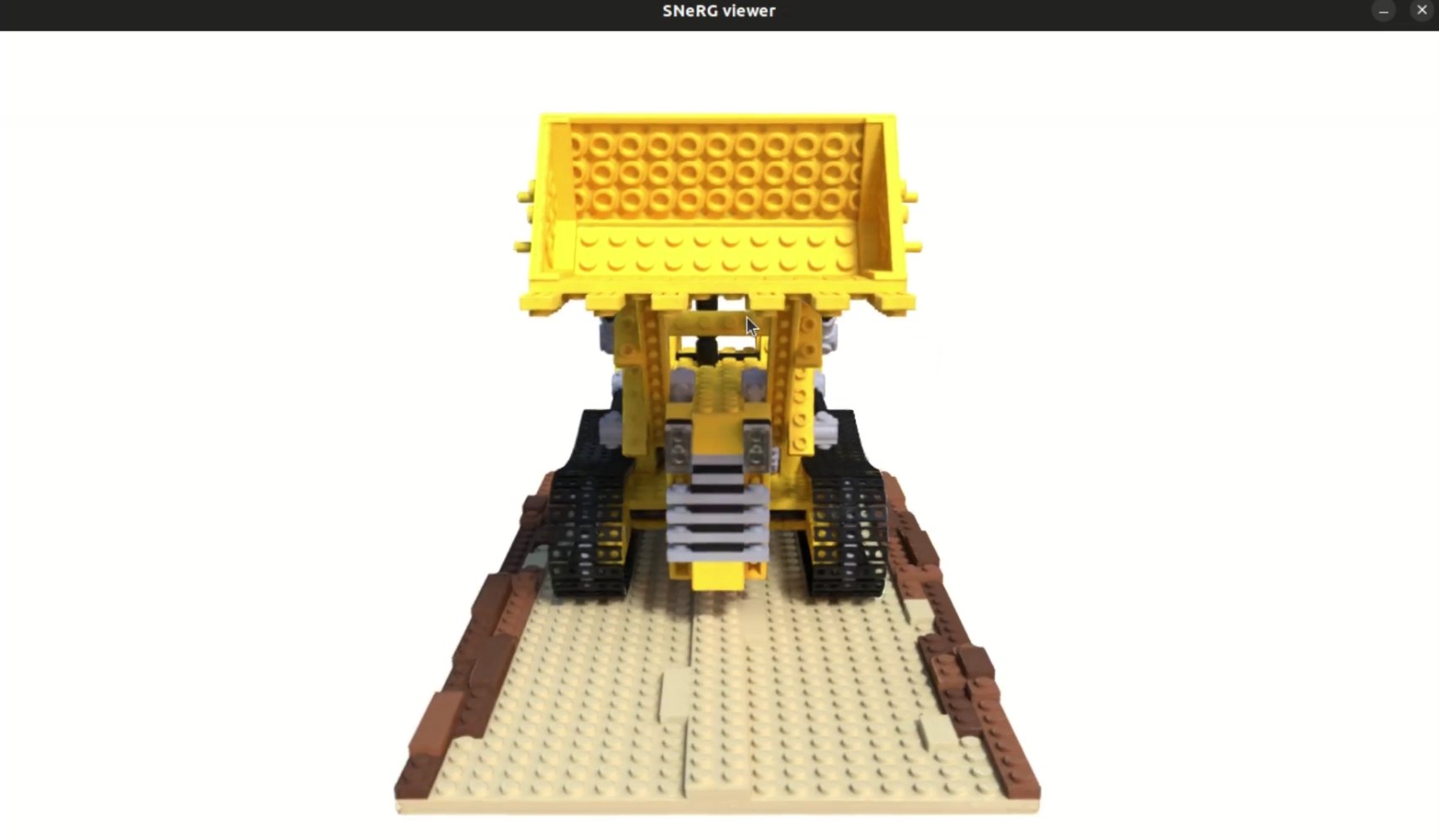
Now whenever we want to create a view of a 3D scene, all we have to do is give the viewing direction and the position as input to the neural network and wait for 5 minutes, and, BAM! we got our output. However, this seems too slow, and absolutely cannot be used for real-time applications like the viewer I made the past week.
So How did I do this?
Sparse Neural Radiance Grid (SNeRG)
This novel representation is introduced in the paper - “Baking Neural Radiance Fields for Real-Time View Synthesis” by the team at Google Research
Basically, they trade storage for speed. We precompute a few stuff and store it into a sparse 3D voxel grid data structure. Each active voxel contains the opacity, diffuse color, and a learned feature vector representing the view-dependent effects.
Modifications to NeRF:
- “deferred” NeRF architecture - View-dependent effects are computed using an MLP that only runs once per pixel instead of once per 3D sample as in the original NeRF architecture
- We need our storage data structure to be sparse, so we need the predicted opacity field to encourage sparsity. This is achieved through regularization
Deferred NeRF architecture
First, we restructure NeRF to output a diffuse RGB color, a 4-dimensional feature vector, and volume density.
To render a pixel,
- Accumulate diffuse colors and feature vectors along each ray
- Pass the accumulated feature vector and color, concatenated with the ray’s direction to a very small MLP (2 layers with 16 channels each)
- Add the output with the diffuse color to produce view-dependent effects
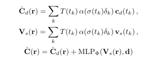
(Source - Baking Neural Radiance Fields for Real-Time View Synthesis - https://arxiv.org/pdf/2103.14645)
Opacity Regularisation
Rendering time and the required storage for a volumetric representation strongly depend on the sparsity of the data structure. To encourage sparsity, we add a regulariser that penalizes predicted density using a Cauchy loss during training.
$$ L_s = \lambda_s \sum_{i,k}log(1 + (\sigma(r_i(t_k))^2/c))$$
This loss is only computed for the coarse samples.
For Reference, To know more about Cauchy Loss - https://arxiv.org/pdf/2302.07238
SNeRG Data Structure
Represents an N^3 voxel grid in a block-sparse format using two smaller dense arrays. The first array is a 3D Texture Atlas containing densely packed “macroblocks” of a fixed size, corresponding to the content. The second array is an (N/B)^3 indirection grid, basically, it stores whether a block is empty or stores an index that points to the corresponding content in the 3D texture atlas.
Rendering
The critical differences are as follows:
- Precompute the diffuse colors and feature vectors at each 3D location, which allows us to look them up within our data structure
- Instead of evaluating the MLP for each 3D sample, we can infer it once per view-dependent effects
To minimize the storage cost and rendering time, only allocate storage for voxels in the scene that are both non-empty and visible in at least one of the training views.
To know more about the SNeRG Data Structure, I would recommend you to have a look at the paper - https://arxiv.org/pdf/2103.14645
Using the above principles, I wrote a program in OpenGL and C++, to view the models. The 3D atlas, Indirection Grid, and Model Weights will be passed to the shader as uniforms. There is a quite a lot of interesting graphics and rendering concepts involved in OpenGL. However, it is a topic for another day.
If you want to start learning openGL, you could start here - https://learnopengl.com/Introduction